Excel SUM Formula: The Ultimate Guide to Adding Values
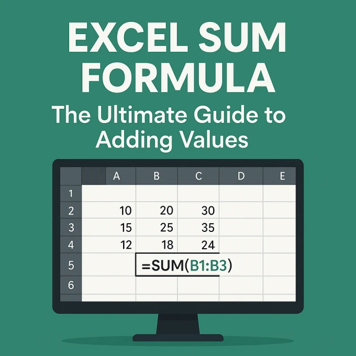
Learn everything you need to know about the SUM formula in Excel, from basic usage to advanced techniques.
The SUM formula in Excel is used to add numerical values together. It's one of the most fundamental and frequently used functions in Excel. It's versatile and can handle various types of input, including numbers, cell references, ranges, and even other formulas.
The basic syntax of the SUM formula is as follows:
=SUM(number1, [number2], ...)number1: The first number or cell reference you want to add. This is required.[number2], ...: Optional. Additional numbers or cell references you want to add. You can include up to 255 arguments.To add two numbers directly, enter the following formula into a cell:
=SUM(10, 5)This will display 15 in the cell.
A more common use case is to add the values contained in specific cells. Let's say cell A1 contains 10 and cell A2 contains 5. You can use the following formula:
=SUM(A1, A2)This will also display 15 in the cell where the formula is entered.
To add all the values within a range of cells, use the colon (:) operator:
=SUM(A1:A10)This will add the values in cells A1 through A10.
You can combine ranges, individual cells, and numbers within a single SUM formula:
=SUM(A1:A5, B2, 10, C1:C3)This will add the values in the range A1:A5, the value in cell B2, the number 10, and the values in the range C1:C3.
Excel provides a convenient feature called "AutoSum" that automatically suggests a range to sum. Here's how to use it:
| Item | Cost |
|---|---|
| Apples | 2 |
| Bananas | 3 |
| Oranges | 4 |
| Total | =SUM(B2:B4) |
The SUMIF formula allows you to sum values in a range based on a specific criteria. The syntax is:
=SUMIF(range, criteria, [sum_range])range: The range of cells you want to evaluate against the criteria.criteria: The condition that determines which cells will be summed.[sum_range]: Optional. The range of cells to sum. If omitted, the 'range' is summed.Example: Suppose you have a list of sales, and you want to sum the sales only for a specific product, "Widgets".
=SUMIF(A1:A10, "Widgets", B1:B10)This formula will sum the values in B1:B10 only if the corresponding cell in A1:A10 contains "Widgets".
The SUMIFS formula extends SUMIF by allowing you to sum values based on multiple criteria. The syntax is:
=SUMIFS(sum_range, criteria_range1, criteria1, [criteria_range2, criteria2], ...)sum_range: The range of cells to sum.criteria_range1: The first range of cells you want to evaluate against a criteria.criteria1: The first condition that determines which cells will be summed.[criteria_range2, criteria2], ...: Optional. Additional criteria ranges and criteria.Example: Suppose you want to sum the sales for "Widgets" sold in the "East" region.
=SUMIFS(C1:C10, A1:A10, "Widgets", B1:B10, "East")This formula will sum the values in C1:C10 only if the corresponding cell in A1:A10 contains "Widgets" AND the corresponding cell in B1:B10 contains "East".
While SUMIF and SUMIFS are generally preferred, you can sometimes use SUM with array formulas to achieve complex conditional summing. These formulas often require pressing Ctrl+Shift+Enter (CSE) to enter them correctly. (Note: Modern Excel versions often handle array calculations without needing CSE.)
Example: Equivalent to the SUMIF example above:
=SUM((A1:A10="Widgets")*(B1:B10))This formula multiplies a boolean array (TRUE/FALSE) created by the condition (A1:A10="Widgets") with the values in B1:B10. TRUE is treated as 1 and FALSE as 0, effectively summing only the rows where the condition is met.
Important: Array formulas can be computationally intensive, especially with large datasets. Use SUMIF or SUMIFS when possible for better performance.
#VALUE! ErrorThis error usually occurs when one or more of the cells being summed contains text or an error value. Make sure all cells within the range contain valid numbers.
Double-check the range you're summing to ensure it includes all the desired cells and excludes any unintended cells. Also, verify that the cells contain the correct values.
Sometimes, cells might appear to contain numbers but are actually formatted as text. Select the cells and change the format to "Number" or "General" in the "Number" group on the "Home" tab.
A circular reference occurs when a formula refers to its own cell, either directly or indirectly. This can lead to incorrect results or Excel displaying a warning message. Review your formulas carefully to avoid circular references.
=SUM(A1:A10), you could use =SUM(SalesData) if you've named the range A1:A10 as "SalesData".